This is a the result of the second project of CS194-26 from Fall 2020
1.1: Finite Difference Operators
We compute the magnitude of the gradient by first finding the gradient in the x and y directions, dx and dy respectively, then computing (dx**2 + dy**2)**0.5 to get the true magnitude.
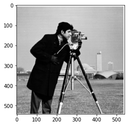
For the following image:
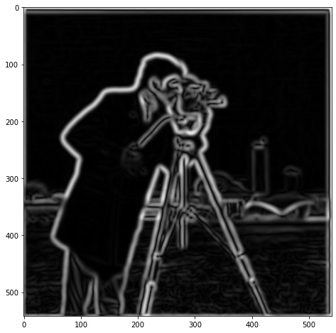
The squared magnitude of the gradient is shown below.
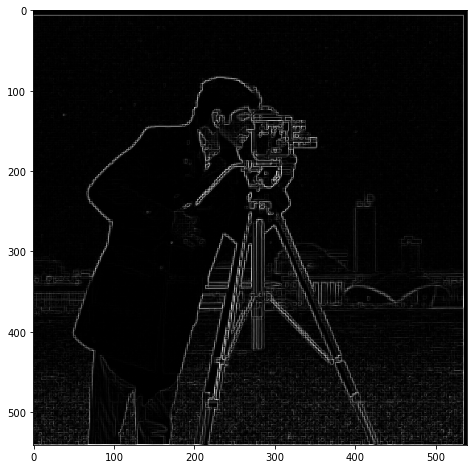
The problem with this specific method is that we get a fair amount of noise: we want the edges of the image but the gradient still has a significant value in smaller places such as the grass. If we look at a histogram of the squared gradient we see that there are a fair number of small values.
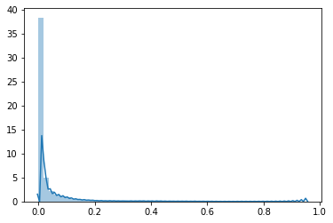
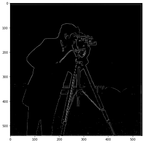
So we can simply threshold these out and we get something slightly cleaner:
1.2: Derivative of Gaussian:
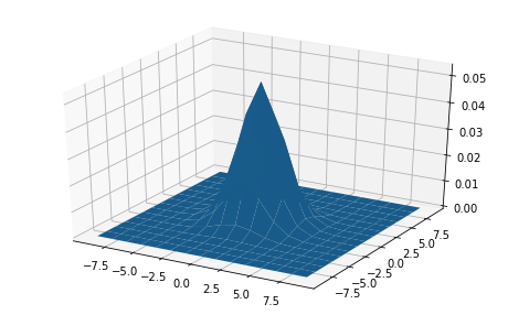
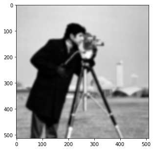
Another way to get the true edges would be to first denoise the image using a gaussian filter:
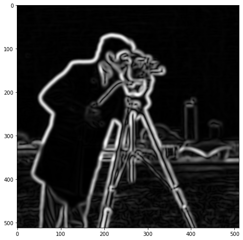
And then compute the gradient on this resulting image:
Here we can see this gives us a better representation of edges at the expense of granularity.
 Since this is just two repeated convolutions we can simply convolve the filters in order to get a single filter which computes the x and y gaussian gradients.
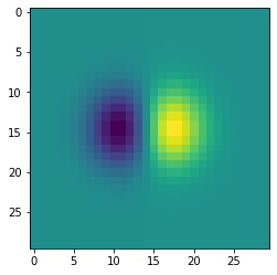
And we can see that this gives us the same result as before
1.3: Image Straightening
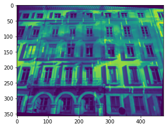
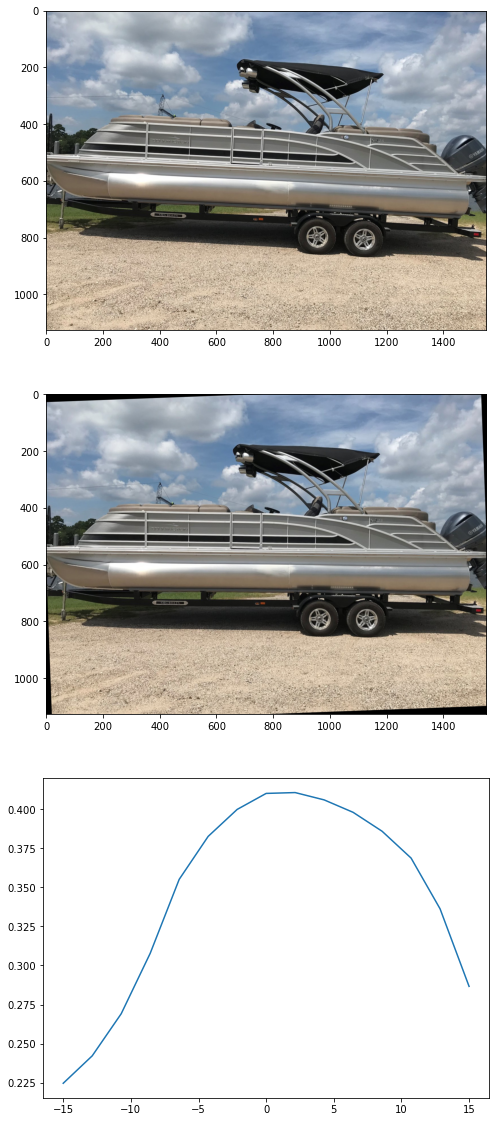
Now we’ll demonstrate how we can use the image gradient for straightening the following image:
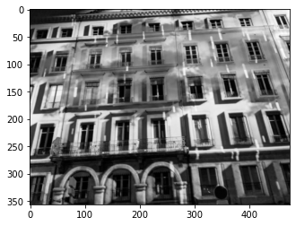
Instead of looking at the magnitude of the gradient, we will instead look at the angle of it, given by theta = arctan(dy/dx).
This will tell us what the angle of the gradient is in a given region and thus what a given edge is like (we can do this in addition to filtering out low magnitude gradients to prioritize edges).
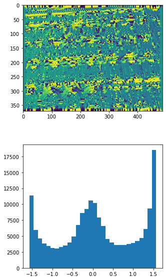
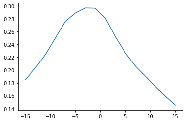
Here is the theta for the above image and the distribution of angles.
We can see it’s just slightly off at 0 and at pi/2 and -pi/2.
We want to maximize how close this is to those angles so we count the number of points with angles whose absolute value are close to 0, pi/2.
Rotating between -15 and 15 degrees, we get the following percentage of angles in the given threshold:
 We then choose the image with the highest such amount and look at that specific rotation:
Instead rotating the color version of the image we get:
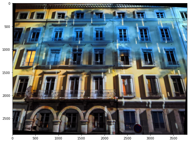
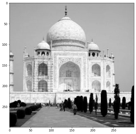
Nice! This works well for images with a fair number of horizontal and vertical edges such as:
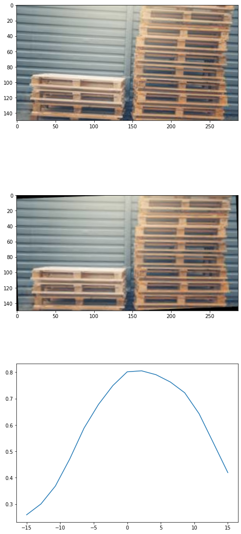 And
And
This does break, however, for images with less common or pronounced vertical and horizonal features such as
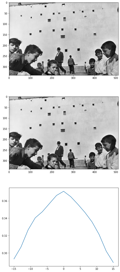 The rotations are likely thrown off by the strong gradients and angles shown on the kids in the foreground even though we can see the wall is slanted in the background.
2.1 Image “Sharpening”
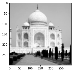
Now let’s play with some filters. First let’s try to sharpen this image:
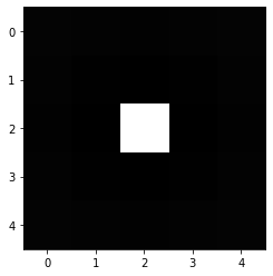
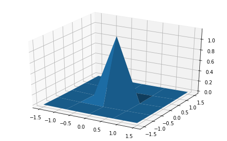
We know we can filter out high frequencies if we use a gaussian kernel such as the 5x5 one below:
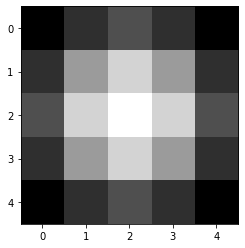
Which gives us a blurred version of the image.
If we subtract this blurred version from the original image, we are left with mostly high frequencies in our image:
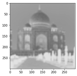
Hence adding it back with some scaling factor will give us a “sharper” version of the image, in which the higher frequencies make the image seem sharper.
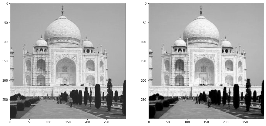
The sharpenend image is on the left in this image.

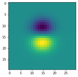
We can also combine this into a single filter by combining the unit impulse filter with the gaussian to get the laplacian:
And we see that using just this filter gives us the same result. Sweet!
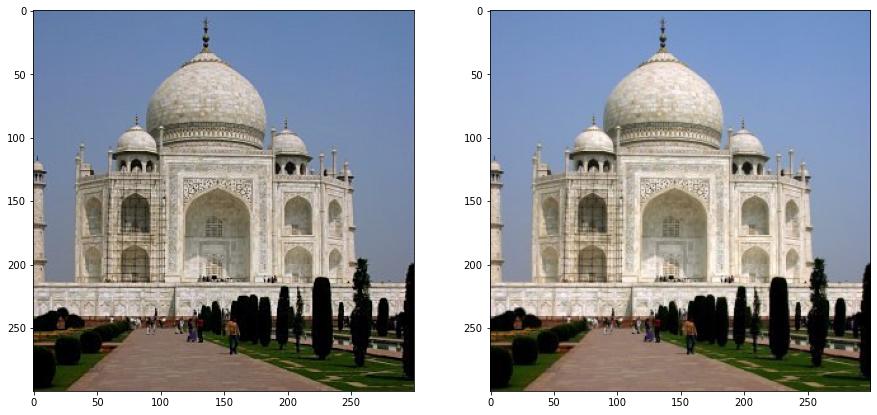
Done per-channel on the color image looks a little strange but generally seems to work:
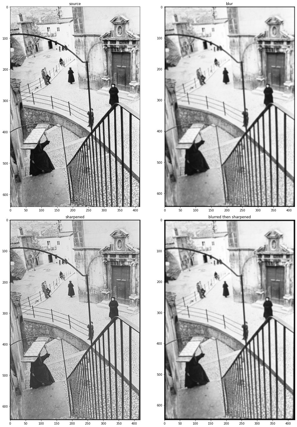
Here it is applied to a Henri Cartier-Bresson shot. We can see a significant effect of sharpening.
If, however, we try to sharpen after blurring, it doesn’t have much effect.
This is due to the fact that we have little by the way of high frequencies to add back in, as applying the gaussian filters many of them out.
2.2 Hybrid Images
We can use our techniques of high and low frequency manipulation to make images which appear to be different depending on how far away they are seen.
Consider the following aligned images.
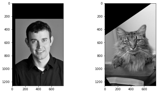
We can overlay these by taking the high frequencies from one and the low from the other using our gaussian filter.
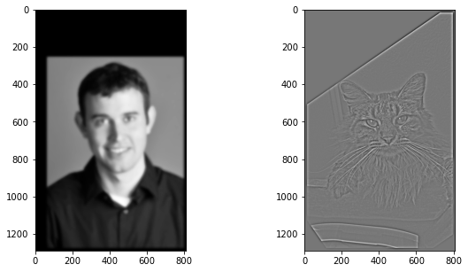
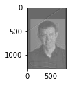
Combining these images linearly we get
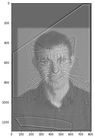
Which while large looks like a cat, at a small view looks like our good friend Derek.
I for some reason felt compelled to combine the following two images of Rick and Alyosha.
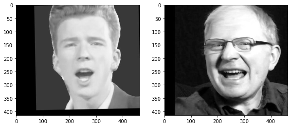
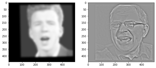
Which yields the following beauty:
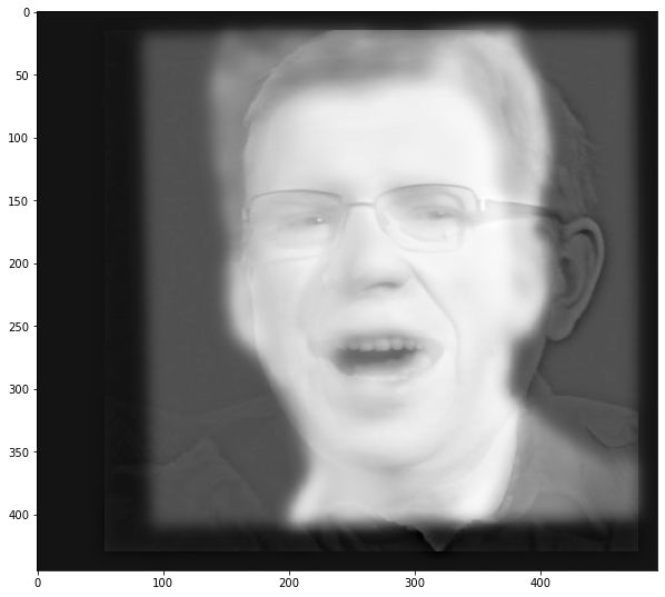
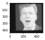
That when seen from afar looks just like Rick!
We can look at how these images are represented in the frequency domain using the log absolute value of the fourier transform:
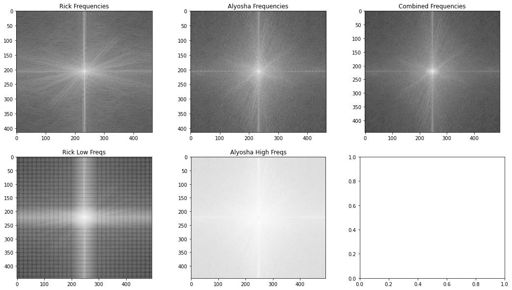
If we look at the frequency representation of the combined image, we see that the higher frequencies (those further from the center) are far more like Alyosha’s frequencies than Rick’s.
It might be difficult to see, but the lower frequencies are also more similar to ricks.
The bottom two images are the fourier transforms of the respectively filtered images, which aren’t particularly illuminating (I think the artifacting in Rick’s image is from the weird way I cropped it).
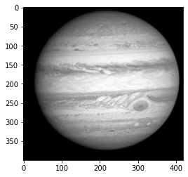
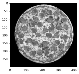
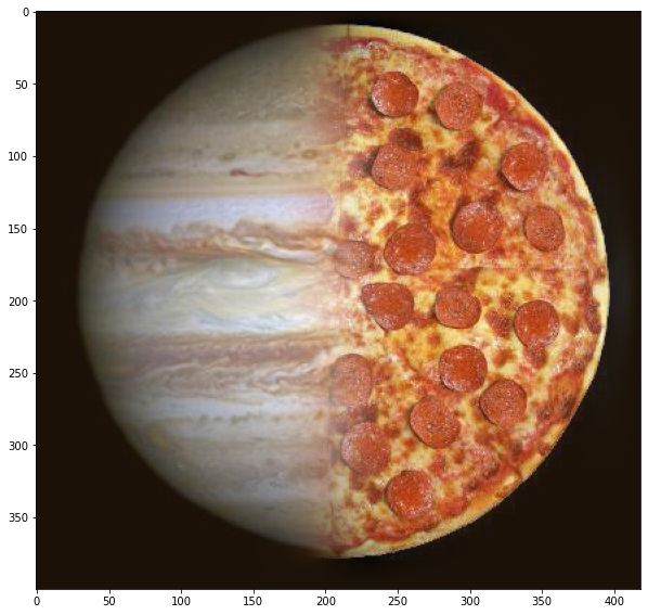
In quarantine I have missed going one of my favourite restaurants in Berkeley, the infamous pizza place Jupiter. The following images are dedicated to the BBQ Chicken pizza at Jupiter.
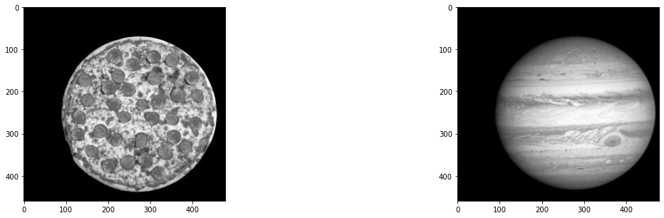
Oh wow look a cool planet!
Oh wow look a tasty pizza!
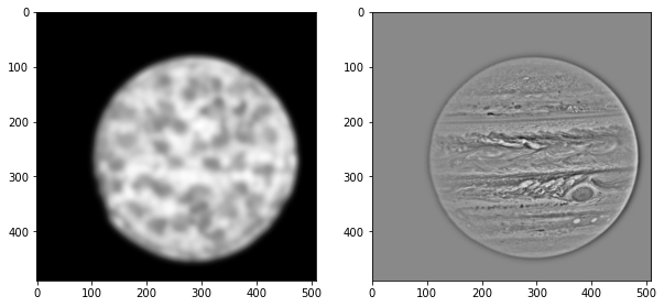
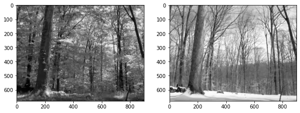
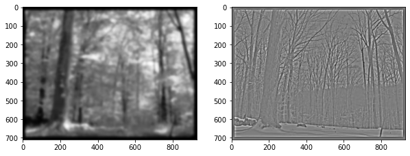
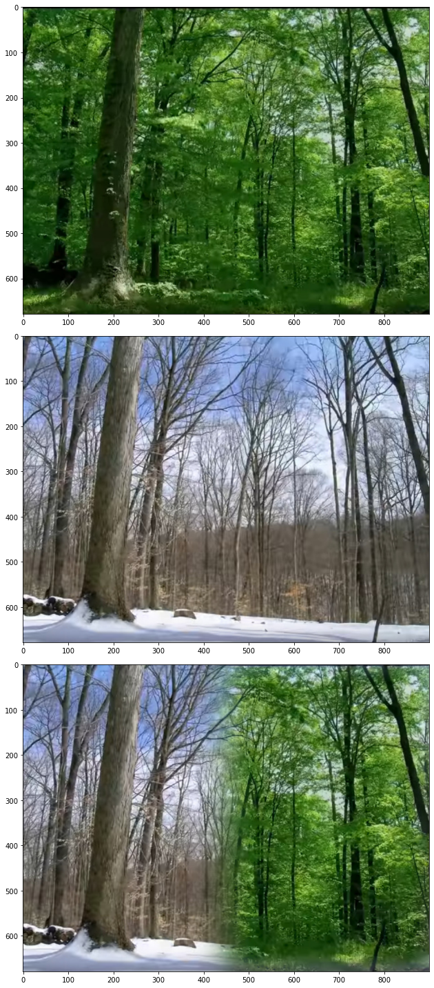
This works great in both above examples as we can discern the low frequency image by its low frequencies and the high frequency image by its high frequencies. If we can’t do this, we don’t get the same effect. Consider my following attempt to mix a snowy and leafy forest:
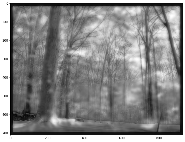
 !
!
None of them really look like much, as we can’t discern the leafy forest by its low frequencies or the snowy one by its high frequencies.
2.3: Gaussian and Laplacian Stacks
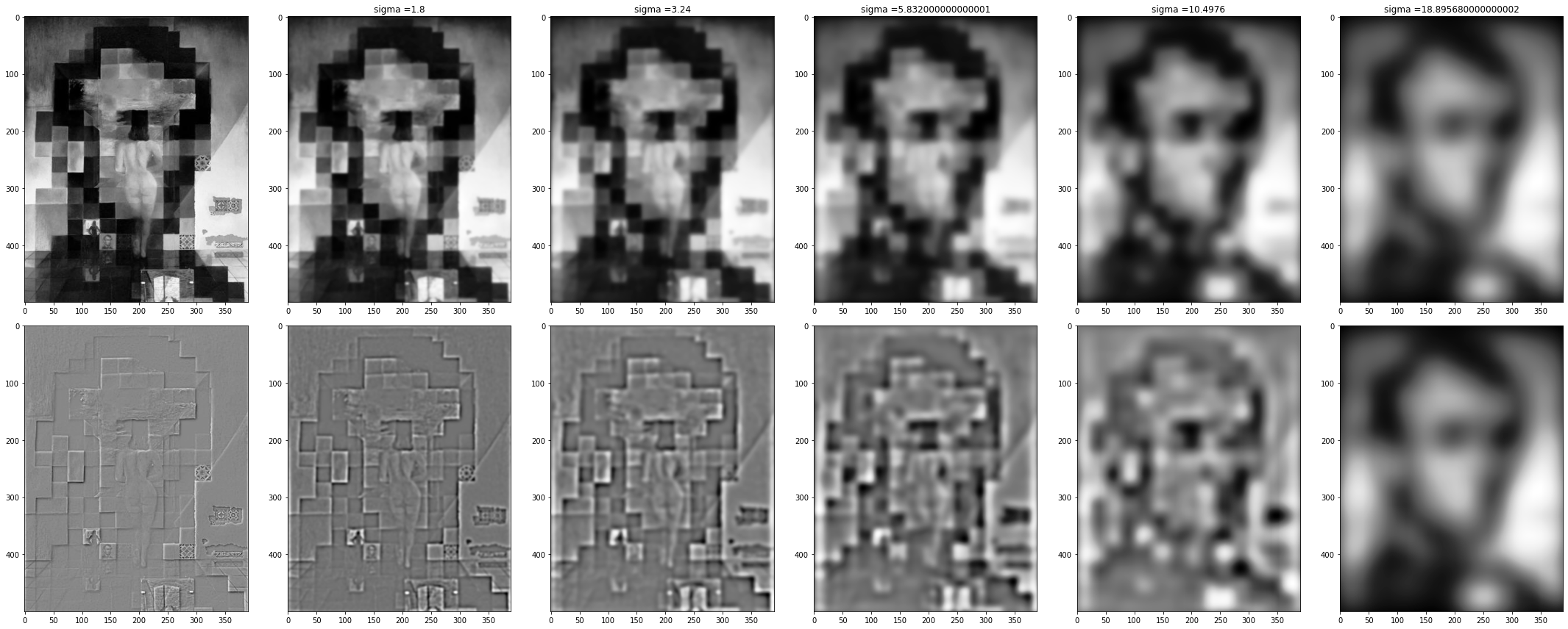
We can also use progressively higher variance gaussians to get a perspective of different levels of frequencies in an image. For example, the following image has low frequencies that look like Lincoln while it’s high and medium frequencies look like a lady in front of a mural.
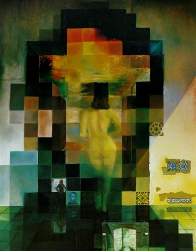 The Gaussian and Laplacian stacks show this perfectly, with only Lincoln present the lowest frequencies, the blocks of the mural in the high frequencies, and the woman primarily in the middle frequencies.
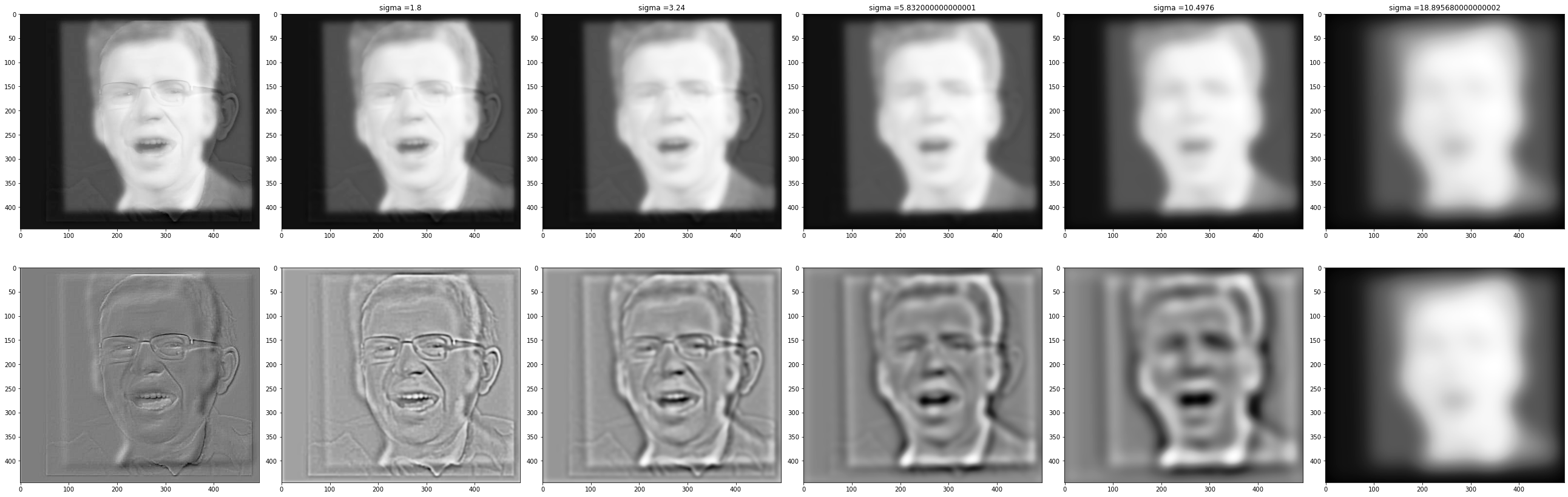
This can also demonstrate the effect on our friend Rickyosha. We see mostly the texture of Alyosha in the highest frequencies and only the shape of Rick in the lowest frequencies (note that you may have to open this image separately as it may be too small to properly see the high frequencies in the bottom left).
2.4: Multiresolution Blending
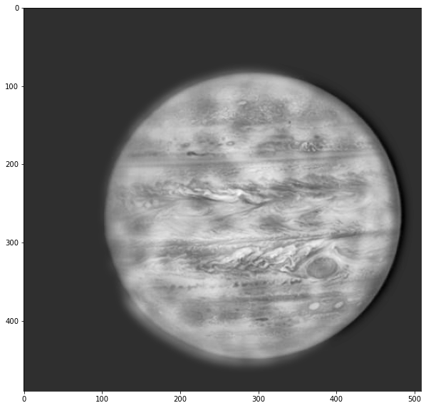
Oh, you didn’t think I had forgotten about Jupiter yet, did you? Let’s blend these two images cleanly using more of our frequency techniques!
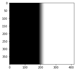
Here we’ll use the following mask (just a simple linear step function) and pass it through a Gaussian stack as above.
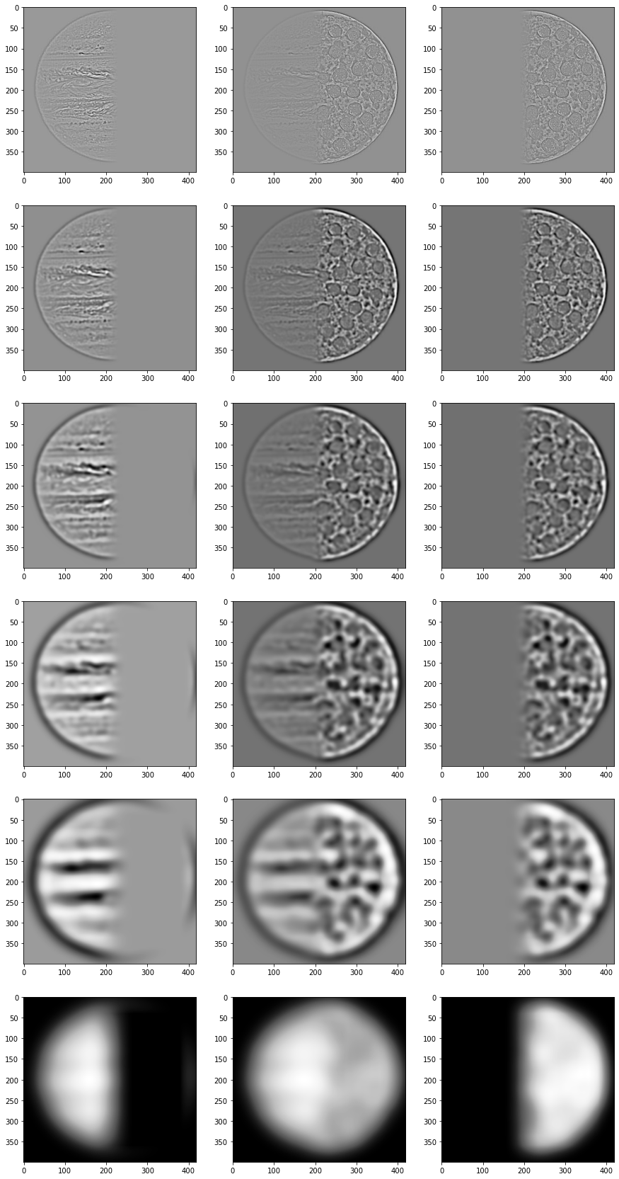
We’ll also compute the laplacian stacks for both the Jupiter and pizza to get different bands of frequencies.
We will then combine these with the gaussian-stacked mask to get a wide blend for low frequencies and a closer blend for high frequencies!
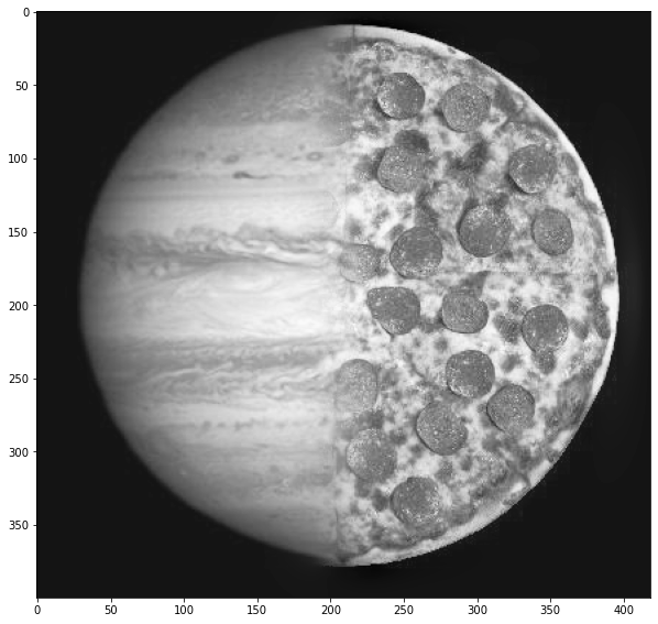
If we sum up all these blended images, we get the following… tasty… tasty… image…
We can simply apply this per channel to get an even more.. oh.. mmmm..
Could we also use this technique to combine our snowy/leafy example which failed above?
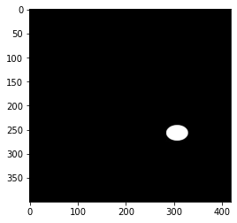
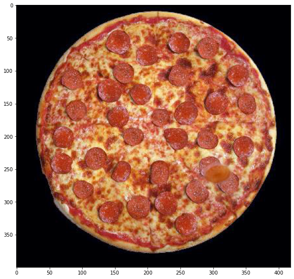
 Wow, looks awesome! We aren’t limited to just a vertical mask though. Let’s try something fancy: let’s put that pepperoni-looking spot on jupiter on our pepperoni pizza using the following mask:
 Looks nice and smooth
Takeaways
I definitely learned the utility of gaussian filters as low-pass filters. I previously thought the most reasonable way to do such a thing would be to clip the fft of an image, but this works shockingly well and produces some pretty cool results!